Grammar of Graphics in Brookings Style • ggbrookings

Overview

ggbrookings is a ggplot2 extension which implements the Brookings style guide. It offers several color palettes, a custom theme, and a few helper functions.

Installation

In order to install packages from GitHub you need to install the remotes package. If you’re using a Windows computer you will also need to install RTools, which is available here and on the software center if you’re using a Brookings laptop.

install.packages("remotes")
remotes::install_github("BrookingsInstitution/ggbrookings", build_vignettes = TRUE)

Note: If you are on a Brookings laptop, you may need to change your timezone for devtools to work. This can be done by running:

Sys.setenv(TZ = 'UTC')

Fonts

Inter is Brooking’s main font. You will need to install it by visiting Google fonts and clicking “Download family”.

Once you’ve done this, unzip and open each of the .ttf files and click install. Finaly, run the code chunk below to ensure Roboto is imported and registered:

import_inter()

If you run into any problems while installing fonts on a Windows computer try the following solution from this issue:

remove.packages("Rttf2pt1")
remotes::install_version("Rttf2pt1", version = "1.3.8")

Usage

Currently, the ggbrookings package only has a few simple user facing functions:

theme_brookings() overrides the default ggplot2 theme for a custom one which adheres to the Brookings style guide.
scale_color_brookings() and scale_fill_brookings() provide several color palettes that are consistent with the Brookings brand and designed to provide color accessiblity.
brookings_view_palette() is a helper function to see the colors from each palette and extract their hex codes.
add_logo() adds a program/center logo to your plots after saving them. See the vignette on adding logos for more details.

Examples

I highly recommend that you install librarian by running install.packages('librarian') as it lets you quickly install, update, and attach packages from CRAN, GitHub, and Bioconductor in one function call.

# Load the necessary libraries
librarian::shelf(tidyverse, palmerpenguins, ggbrookings)

Scatterplot

In order to match the Brookings style in scatterplots you should set geom_point(size = 2) as below:

  ggplot(data = penguins,
       aes(x = bill_length_mm,
           y = bill_depth_mm,
           group = species)) +
  geom_point(aes(color = species,
                 shape = species),
             size = 2,
             alpha = 0.8) +
  geom_smooth(method = "lm", se = FALSE, aes(color = species)) +
  theme_brookings() +
  scale_color_brookings(palette = "misc") +
  labs(title = "Penguin bill dimensions",
       subtitle = "Bill length and depth for Adelie, Chinstrap and Gentoo Penguins at Palmer Station LTER",
       caption = '**Source:** Palmer Penguins',
       tag = 'FIGURE 1',
       x = "Bill length (mm)",
       y = "Bill depth (mm)",
       color = "Penguin species",
       shape = "Penguin species")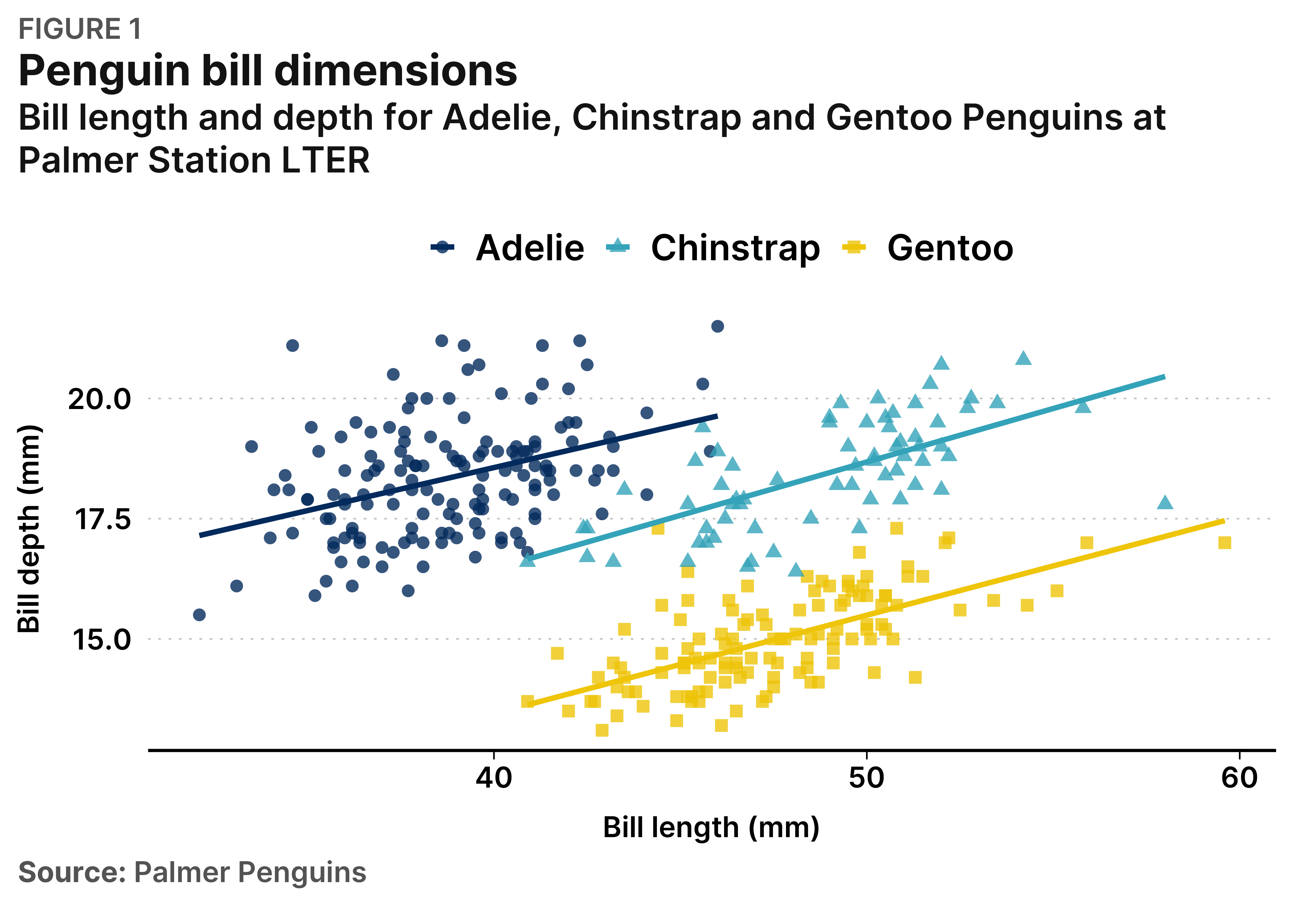

Histogram

  ggplot(data = penguins, aes(x = flipper_length_mm)) +
  geom_histogram(aes(fill = species),
                 alpha = 0.5,
                 position = "identity",
                 bins = 30) +
  scale_fill_brookings(palette = "semantic3") +
  theme_brookings() +
  labs(x = "Flipper length (mm)",
       y = "Frequency",
       title = "Penguin flipper lengths",
       caption = '**Source:** Palmer Penguins',
       tag = 'FIGURE 2') +
    scale_x_continuous(expand = expansion()) +
    scale_y_continuous(expand = expansion())

You can change the size of your text proportionally by setting theme_brookings(base_size = your_size) as shown below:

Faceting

  ggplot(penguins, aes(x = flipper_length_mm,
                     y = body_mass_g)) +
  geom_point(aes(color = sex),
             size = 2,
             show.legend = FALSE) +
  theme_brookings() +
  scale_color_brookings('brand1', na.translate = FALSE) +
  labs(title = "Penguin flipper and body mass",
       subtitle = "Dimensions for <span style = 'color:#FF9E1B;'>**male**</span> and <span style = 'color:#003A79;'>**female**</span> Adelie, Chinstrap and Gentoo Penguins at Palmer Station LTER",
       caption = '**Source:** Palmer Penguins',
       tag = 'FIGURE 3',
       x = "Flipper length (mm)",
       y = "Body mass (g)",
       color = "Penguin sex") +
  facet_wrap(. ~ species, nrow = 3, ncol = 1) +
        scale_x_continuous(expand = expansion()) +
    scale_y_continuous(expand = expansion())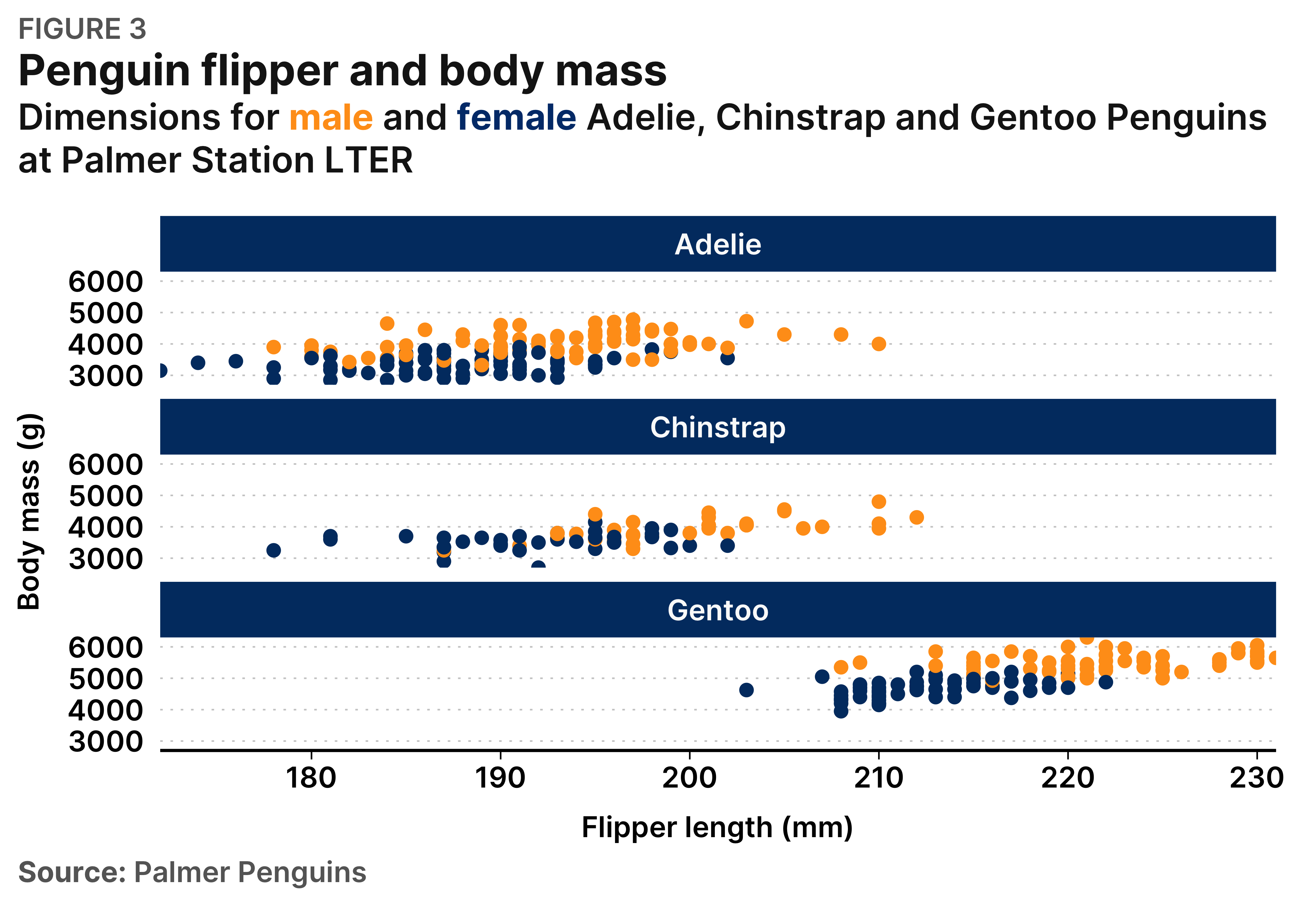

Line plot

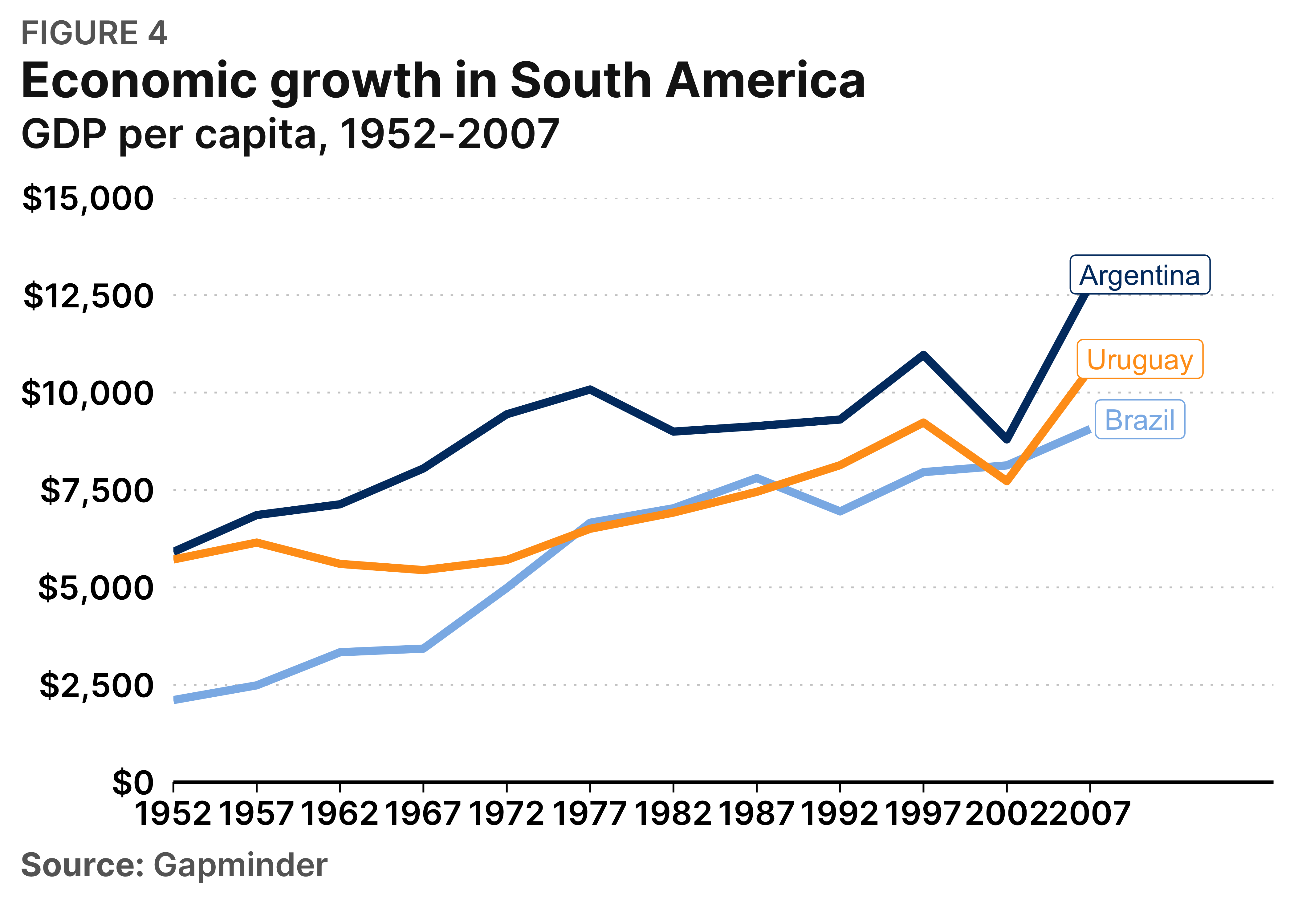
In order to match the Brookings style in line plots you should set geom_line(size = 1.5) as below:

librarian::shelf(gapminder)

gapminder_filtered <-
  gapminder %>% 
  filter(country %in% c('Argentina', 'Brazil', 'Uruguay'))  

gapminder_filtered %>% 
  ggplot(aes(x = year, gdpPercap, color = country, label = country)) +
  geom_line(size = 1.5) +
  geom_label(data = gapminder_filtered %>% filter(year == last(year)), 
             aes(label = country, 
                 x = year + 3, 
                 y = gdpPercap + 250, 
                 color = country)) +
  theme_brookings(base_size = 16) +
  guides(color = 'none') +
  scale_x_continuous(breaks = seq(1952, 2007, 5),
                     limits  = c(1952, 2012),
                     expand = expansion(mult = c(0, 0.1))) +
  scale_y_continuous(labels = scales::label_dollar(), 
                     limits = c(0, 15000), breaks = seq(0, 15000, 2500),
                     expand = expansion(0)) +
  scale_color_brookings() +
  labs(title = 'Economic growth in South America',
       subtitle = 'GDP per capita, 1952-2007',
       caption = '**Source:** Gapminder',
       tag = 'FIGURE 4',
       x = NULL, 
       y = NULL)